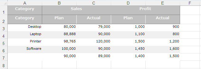
Honesty, the Alteryx is not good at outputting the formatted Excel sheet by itself. For example, if you need 2 rows header, the Table tool can’t do anything. So in order to do that, you usually overwrite the pre-formatted Excel sheet.
However, this time I would like to try making the table with 2 rows header.
What we want to make is…
What we want to make is the header part as follows.

This header has the 1st row that has three column names “Category”, “Sales” and “profit”, but actually there are 6 fields and at the 2nd row thare are 6 fields. In other hands, it means that the Column “A” and “B” is merged, the Column “C” and “D”, “E” and “F” are also merged.
How do you create a two-level header in the first row using the Table tool?
Creat a two-level header
To creat a two-level header, you need to use 2 Table tools.
1. Prepare the data for header
First, you need to prepare the data for the header as follows.

In this case, you need to prepare it at the data part not header part.
2. Add the Table tools
And then, connect the Table tools after each Text Input tools.

At the each Table tools, you need to uncheck the “Show Column Headings” check box. After that, this will prevent unnecessary headers from being displayed.

In other words, each will be displayed as follows.


3. Join by the Union Tool
Join these tables by the Union tool.

At the Union tool, you need to pay attention for the union order. “1st header” should be always coming to the Union tool for the first. Basically, when you connect any tool to the Union tool at first, the connecter is named as #1. Second connecter is named as #2. And normally the data typically arrives in those numerical order. However you can control the data order using “Set a Specific Output Order” option if you want. But this option makes running speed slowly because it makes the Union tool “Blocking tool”. The reason why is “Blocking tool” hold the data and wait until whole data coming.

At this point, the output will look like this:

Please see the output carefully, the vertical line is not match.
4. Add the Layout tool
Next, in order to match the vertical line, use the Layout tool.

The setting of the Layout tool is as follows.

Please see the “Layout Mode” and “Orientation”.
“Layout Mode” should be chosen “Each Group Of Records” or “All Records Combined”. This will combine what was separate in each record into a single record.
And also, “Orientation” should be chosen “Vertical Merge Contents to Line up Table Columns”. This is an important point. This makes the vertical cell position matched.

Here, Alteryx neatly aligns them to even intervals. In other words, for every two items on the second line, there is one item on the first line.
And then, output the Excel using the Rendering tool, you can see the output below. The column A and B, C and D, E and F are merged cells.

If you want to design the header, you can set the Table tools’s setting which you like.

Important notice
The header has odd Number
The way that I explained in this post is depending on the number of header and its position. The sample that I explained has 6 columns, each with 2 columns. However how about the another pattern as follows?

If you do the same way that I expained, it doesn’t work well.

In this case, you can use dummy column as follows.

After do that, you can fix the position of “Plan” column, but it has unnecessory column.

Now what I can do is all. If you have better way, please let me know.
If it doesn’t work well
I think that there are many patterns so that sometimes you can’t adjust the setting. Honesty, in that case, you need try and error. As I said first, Alteryx is not good for those situation. I just explained a simple pattern to do that.
Can we merge the cells vertically?
Unfortunately, you can not merge the cells vertically. If you want, I think that you can use the empty cells for that purpose.
Sample workflow download
Next Blog post
The next blog post is the subsequent of this content. I will explain about data part.


コメント